


Previous part:

Suppose you operate a web-service across three data centres. One region handles a large share of the traffic, and then it disappears.
Your monitoring detects failed health checks. The load balancer stops sending new requests to the failed region. Queues hold work that cannot be processed immediately. Clients retry some requests. Spare capacity in the remaining regions absorbs part of the load, autoscaling adds more instances, and operators receive alerts while the system settles into a degraded but usable state.
Software engineers know this story. We design distributed systems with observability, redundancy, failure detection, isolation, automated recovery and human escalation because components eventually fail.
Now replace the data centre with a 1,000 MW generator connected to the European power grid.
The comparison still helps, but the failure is harder. Electricity cannot wait inside a queue until another generator is ready. Consumers continue withdrawing power at the same moment that generation disappears. The electrical state begins changing before a monitoring system has delivered the first alarm, and power redistributes through transmission lines according to physical laws rather than routes selected by an application.
The grid also has shared physical state. Frequency reflects the balance between active power generation and consumption. Voltage differs across the network and depends strongly on local reactive power and power flows. Current, equipment temperatures, rotor angles and line loading continue changing while software is still collecting measurements.
In Part 1, Electricity Is Not Water, we built the physical model behind generators, transformers, AC and frequency. In Part 2, The Grid Is Not a Pipeline, we assembled the network as a graph of substations, lines, generators, storage and loads. Now the machine is running, and we can ask how it stays alive when its state never stops changing.
In this post you will learn how protection, monitoring, operation and control work together, what SCADA contributes to that chain, which physical variables operators care about, and what happens from the first instant after a large generator disconnects until the grid reaches a new secure state.
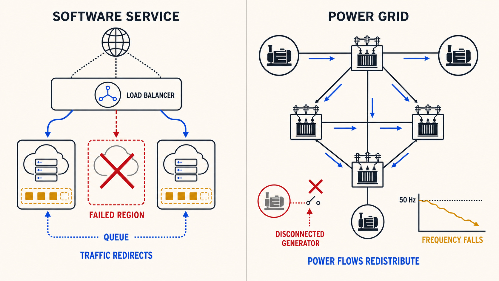
Figure 1: A software platform can queue and redirect work. A power-system disturbance begins changing the shared physical state immediately.
A Distributed Physical System
The grid behaves like a distributed system in the broad sense. It spans many locations, has no single machine that contains its complete state, depends on communication and coordination, and must continue operating when individual components become unavailable.
The difference is that its nodes are coupled by physics.
A web service can often tolerate short disagreement between replicas. Messages can arrive late, requests can wait, and a control plane can calculate a new routing decision before the data plane changes. The electrical grid has far less freedom. A breaker opening in one substation immediately changes the topology seen by the electrical system. Voltages and currents respond at electromagnetic speed, rotating machines accelerate or decelerate, and power flows settle into new paths throughout the connected network.
This makes grid stability a broader idea than keeping the lights on. The system must remain within several limits at the same time.
Generation and load balance
A load is anything withdrawing electrical power from the grid. It may be one motor, a railway, a steel plant, a house or the combined demand of an entire distribution network.
Generators—and storage systems when discharging—inject active power, measured in watts. Active power is the average rate at which electrical energy is transferred into net work or heat: it turns motors, warms heaters, moves pumps and powers computers.
Across a synchronous AC system, generation and other active-power injections must continuously match consumption and network losses. When consumption and losses require more active power than generators and other resources provide, energy is initially drawn from the rotating masses of connected machines and frequency falls. When injections exceed consumption and losses, those machines accelerate and frequency rises.
In Continental Europe the target is 50 Hz. Frequency is therefore both a controlled quantity and a system-wide symptom. It tells operators that the active-power balance has changed, although it does not by itself reveal where the cause is located.
Voltage and reactive power
Every connection point in the grid also has a voltage. Voltage can be thought of as the electrical potential that drives current and allows power to move, but operationally the key point is simpler: voltage must stay within an acceptable range at every important bus and connection point.
Frequency is broadly shared across a synchronous area. Voltage is local. A bus in western Austria, a substation near Vienna and an interconnector in Germany can all have different voltage magnitudes at the same moment.
AC equipment needs changing electric and magnetic fields. Part of the current repeatedly stores energy in those fields and returns it later in the AC cycle. The associated quantity is reactive power, measured in var. It does not produce net work over a complete cycle, but it still creates current, occupies network capacity and affects voltage.
When an area lacks reactive-power support, voltage tends to fall. When it has too much, voltage can rise. The relationship is not perfectly isolated, because active power, reactive power, current, voltage and network impedance affect each other. Still, the following first model is useful:
Active power is closely connected to frequency, while reactive power is closely connected to voltage.
Power flow and transmission capacity
Power flow describes how active and reactive power move through the connected network. In software terms, the grid has a graph, but it has no router assigning each megawatt to a chosen path. Flows emerge from topology, line impedances, voltage magnitudes and phase angles.
If one transmission line opens, the power it carried does not wait for a new route. The electrical state changes and the flow redistributes over the lines that remain. A line far from the original event may receive much of the additional loading.
Each element has operational limits. A conductor can carry only so much current before heating becomes unacceptable. Transformers have thermal and equipment limits. Voltages must stay inside permitted ranges. The system also has stability limits that can become restrictive before a wire reaches its thermal rating.
This is what transmission capacity means operationally. It is not only a fixed number printed on a line specification. The usable capacity depends on the wider network state, including which elements are available, how power is injected and withdrawn, the weather, voltage conditions and what would happen if another component failed.
A grid can have enough total generation and still be unable to transport it safely to the loads that need it. This is why balancing generation and managing network congestion are related tasks, but they are not the same task.
Protection, Operation and Control
When I first tried to understand grid operations, these words blurred together. A relay trips a breaker, an operator opens another breaker, an automatic controller changes generator output, and SCADA displays all three events. It is easy to treat everything as one large control system.
The distinction becomes clearer when we ask what each area is trying to achieve.
Protection detects and isolates danger
A fault is an unintended electrical condition such as a short circuit, an insulation failure or an accidental connection between conductors and ground. Faults can create currents and voltages far outside normal operating values, damage expensive equipment and destabilise the surrounding network.
Protection systems exist to detect these conditions and isolate the affected equipment quickly.
A protection relay receives electrical measurements from instrument transformers or sensors. It applies configured logic to determine whether the measured condition indicates a fault or another dangerous state. Depending on the protected asset, the relay may compare currents entering and leaving a transformer, estimate the apparent distance to a fault on a line, watch for excessive current, or use measurements exchanged with a relay at the other end of the line.
When the relay decides that the equipment must be disconnected, it sends a trip signal to a circuit breaker. The breaker is the heavy electrical switch capable of interrupting normal load current and, within its rating, the much larger current produced by a fault.
The protected network is divided into protection zones around lines, transformers, busbars and generators. These zones usually overlap around breakers so that there is no unprotected gap. The design aims to remove the smallest practical part of the grid while still clearing the fault reliably. Backup protection covers cases where the primary relay, communication path or circuit breaker fails.
Protection is mainly local, automatic and fast. A line fault may need to be cleared within tens of milliseconds. The relay cannot wait for SCADA to send measurements to a control centre, for an operator to interpret an alarm and for a remote command to return. The trip path is designed to work without that sequence.
SCADA will report what happened. Operators will investigate and decide how to restore the network. Those steps matter, but they come after the immediate protection action.
Operation builds and maintains a secure state
Operation is the continuous work of understanding the current grid, preparing it for expected conditions and responding when reality differs from the plan.
Dispatchers in control rooms track the network topology, planned outages, unavailable equipment, generator schedules, weather, load forecasts, active and reactive reserves, voltages and line loading. They coordinate switching, release equipment for maintenance, return it to service, communicate with generators and distribution operators, and exchange information with neighbouring transmission system operators.
Routine work occupies much of this domain. Taking a transformer out of service for maintenance changes the grid before any failure occurs. A dispatcher needs to know whether the remaining network can carry the expected power and whether it can still survive another credible outage.
This leads to contingency analysis, which repeatedly asks questions such as:
What happens if this line trips?
What happens if the largest generator disconnects?
Will another transformer overload?
Will a bus voltage leave its permitted range?
Which remedial actions would still be available?
The common N-1 idea means that the system should normally tolerate the loss of one relevant component without leaving acceptable operating limits after the allowed corrective actions. The exact application is more detailed than that sentence, but the mental model is valuable: operators manage the present while continuously testing possible next states.
EU system-operation rules require TSOs to monitor active and reactive flows, voltages, frequency, reserves, generation and load in real time, and to perform recurring contingency analysis against operational security limits. They also require close-to-real-time analysis to use state estimation. The complete rules are in the EU System Operation Guideline.
Control changes the state
Control is the set of actions that move the grid toward a desired operating state.
Some controls are built into equipment. A generator governor responds to frequency. An automatic voltage regulator changes excitation. A transformer tap changer adjusts its ratio. A capacitor controller switches a bank when voltage crosses a threshold.
Other controls are centralised. Automatic generation control sends changing active-power setpoints to participating resources. A control-room application can request a breaker operation. A dispatcher can instruct a power plant to change active or reactive output, order redispatch, or coordinate a topology change with another operator.
Operation and control therefore describe different parts of the same process. Operation provides the context, objectives and decisions. Control applies physical actions, either automatically or through commands initiated by operators. A protection relay also causes a physical action, but its purpose and logic are different: it removes danger immediately rather than optimising the wider operating state.
A useful software comparison is this:
Protection resembles local safety logic with authority to shut down a dangerous component.
Monitoring provides observability.
Operation resembles the work of site reliability engineers who assess the complete service and choose a recovery strategy.
Control contains the automated loops and commands that change the running system.
The comparison helps organise the responsibilities, although the grid remains coupled by physical laws throughout the whole process.
How the Grid Becomes Visible
A control room may have wall-sized diagrams and dozens of screens, but the operator still does not see the electrical system directly. The displayed grid is constructed from measurements, communication, equipment statuses and models.
The chain begins in the field.
Measurements begin at the equipment
Sensors and instrument transformers measure current and voltage. From these signals, devices calculate active power, reactive power, frequency and other electrical quantities. Breakers and disconnectors provide position indications. Transformers report tap positions, protection devices report trips, and equipment monitoring systems may provide temperatures, pressures and internal alarms.
A measurement always has context. A value needs a timestamp, a source, a unit and a quality indication. A current value from the wrong bay, a breaker state received late, or a voltage measurement marked good when its input circuit has failed can create a convincing but incorrect picture.
Substation devices collect and process data
Inside a substation, intelligent electronic devices, bay controllers, remote terminal units and substation automation systems collect measurements and statuses. Some values are processed locally. Some are stored as events. Some are forwarded to a remote control centre.
These devices may also receive commands. A control centre can request a breaker operation, change a setpoint or switch voltage-control equipment, subject to interlocks and operational procedures.
Protection lives close to this layer, but it should not be confused with telemetry. A protection relay can share measurements and event reports with the automation system while keeping its trip logic local and independent from the normal SCADA path.
Communication networks transport telemetry and commands
Substations and power plants are connected to control centres through operational communication networks. Depending on the system and its age, these links may use fibre, microwave, radio, leased communication services or other channels, often with redundant paths.
Protocols such as IEC 60870-5-104, IEC 61850, DNP3 and vendor-specific interfaces carry measurements, events, statuses and commands across different parts of the chain. The protocol tells us how information is represented and transported. It does not guarantee that the physical measurement is correct or that the model on the receiving side matches the real substation.
SCADA provides the supervisory interface
SCADA stands for Supervisory Control and Data Acquisition. In a grid control centre, it collects telemetry from many remote sites, presents measurements and equipment states, manages alarms and events, stores trends, and provides authorised operators with remote-control functions.
The word supervisory matters. SCADA gives a central view and allows high-level control of dispersed assets. It does not replace local protection, and it does not independently understand every physical consequence of an action.
A SCADA screen may show a one-line diagram in which a breaker appears open, a line is coloured according to its loading and an alarm list reports a generator trip. Behind that screen sits a long chain of measurement circuits, field devices, communication links, protocol gateways, databases, application logic and configuration.
NIST’s Guide to Operational Technology Security describes the same broad SCADA structure: field devices and RTUs or PLCs communicate through wide-area networks with control servers, operator interfaces, engineering workstations and historians in a control centre.
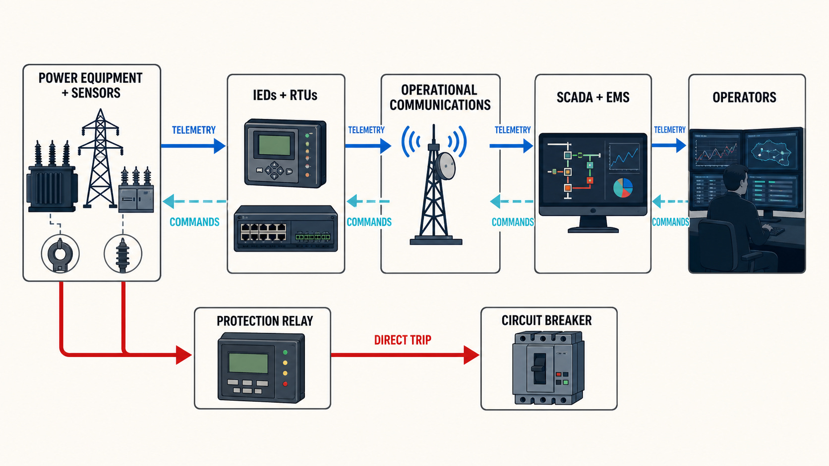
Figure 2: Monitoring information travels toward the control centre, while protection can trip equipment locally without waiting for a remote decision.
Why the screen can be wrong
SCADA is often described as real time, but that does not mean every point reflects physical reality at the same instant.
Measurements are sampled and transmitted at different rates. Communication links can fail. A value can become stale. A breaker indication can disagree with the actual contact position. A substation may be in a temporary configuration that the central model does not yet represent. Sensors have errors, and some values are calculated rather than directly measured.
This creates an observability problem. Operators need enough trustworthy information to determine the state of the network, even when individual measurements are missing or inconsistent.
State estimation reconstructs a coherent picture
State estimation combines telemetry with the electrical network model and the current topology. It checks whether measurements agree with each other, identifies likely bad data and estimates the bus voltages and phase angles that best explain the available information.
The resulting state is still an estimate. Its value comes from making the overall picture more coherent than a raw collection of telemetry points.
This estimated state becomes an input to other Energy Management System applications. Power-flow analysis calculates how power is moving through the network. Contingency analysis simulates possible outages. Security assessment identifies violations of operational limits. Forecasting tools compare the present with expected demand and generation.
Automatic generation control, usually implemented within the European load-frequency control process, uses frequency and control-area interchange information to calculate the area imbalance and adjust participating resources. It does not replace the dispatcher. It performs a continuous control loop inside objectives and limits established by grid operation.
SCADA is therefore a central part of the picture, but it is only one layer. The control room needs telemetry, models, specialised applications, automatic controllers, procedures and experienced operators. Treating the SCADA screen as the grid itself would be like treating a monitoring dashboard as the production system.
What the Grid Must Control
Once the operator has a usable picture of the network, the next question is what can be changed.
There is no single control knob for stability. Different mechanisms influence different parts of the operating state, and changing one variable often affects several others.
Frequency control and reserves
When active-power generation and consumption stop matching, frequency begins to move. The response is organised in layers because no resource is simultaneously instantaneous, unlimited, cheap and available everywhere.
The first physical response comes from stored energy in rotating machines and, increasingly, fast controls in batteries and inverter-based resources. This slows the frequency movement but does not remove the underlying imbalance.
The first organised reserve layer in Continental Europe is Frequency Containment Reserve, or FCR. Participating generators, storage systems and loads monitor frequency locally and change active power automatically. A falling frequency causes upward response, which means more generation or less consumption. A rising frequency causes downward response.
FCR is shared across the synchronous area. Resources respond to the common frequency deviation regardless of which control area caused it. Its immediate purpose is containment: stop the deviation from growing and stabilise frequency.
A reserve is available upward or downward power held by a prequalified resource. The resource might be a hydro plant with headroom, a thermal unit operating below maximum output, a battery with charge available, a pumped-storage plant that can stop pumping, or an industrial load able to reduce consumption. Reserving capacity means keeping part of that flexibility unused during normal operation so it is available when needed.
Once the common response has contained the disturbance, the responsible control area must restore its own balance. Automatic Frequency Restoration Reserve, or aFRR, is activated by the load-frequency controller, often described more generally as automatic generation control. It adjusts selected resources so frequency and scheduled cross-border exchanges move back toward their targets.
If the imbalance is too large or lasts too long, manual Frequency Restoration Reserve, or mFRR, provides another layer. It replaces part of the automatic response and prevents aFRR from remaining occupied indefinitely.
As a concrete Austrian example, Austrian Power Grid’s balancing overview describes FCR as an automatic response that must reach full activation within 30 seconds when the frequency deviation reaches 0.2 Hz. APG states that aFRR must activate within five minutes in the Austrian control area, while automatic and manual restoration reserves together must cover foreseeable balancing errors within 15 minutes. The exact products and rules belong to the European balancing framework and national implementation, but the sequence is the important part:
Slow the frequency change.
Contain the deviation.
Restore the responsible control area.
Replace the used reserves and prepare for another event.
Voltage control and reactive power
Frequency control works across the synchronous system. Voltage control is more local because voltage differs between buses and because transporting reactive power over long distances consumes current and network capacity.
Synchronous generators regulate voltage through their excitation systems. Increasing excitation allows a generator to supply more reactive power within its capability limits, while reducing excitation can make it absorb reactive power. Power-electronic converters can also provide controlled reactive current, although their capability depends on their design, current limits and active-power operating point.
Transformer tap changers adjust the turns ratio and therefore the voltage relationship between network levels. They are useful for maintaining a downstream voltage, but they do not create missing power. Under stressed conditions, repeatedly raising a distribution-side voltage can increase the demand seen by an already weak transmission system, which is why tap control may need to be coordinated or blocked during a voltage emergency.
Capacitor banks supply reactive power and tend to support local voltage. Reactors absorb reactive power and help reduce excessive voltage, especially on lightly loaded high-voltage lines and cables. Devices such as STATCOMs and synchronous condensers provide dynamic reactive-power support when voltage needs to change quickly.
The EU System Operation Guideline treats voltage and reactive-power management as a direct operational responsibility. It lists
transformer tap changes, capacitor and reactor switching, power-electronic devices, generator reactive-power setpoints and coordinated actions with distribution operators among the available remedial actions.
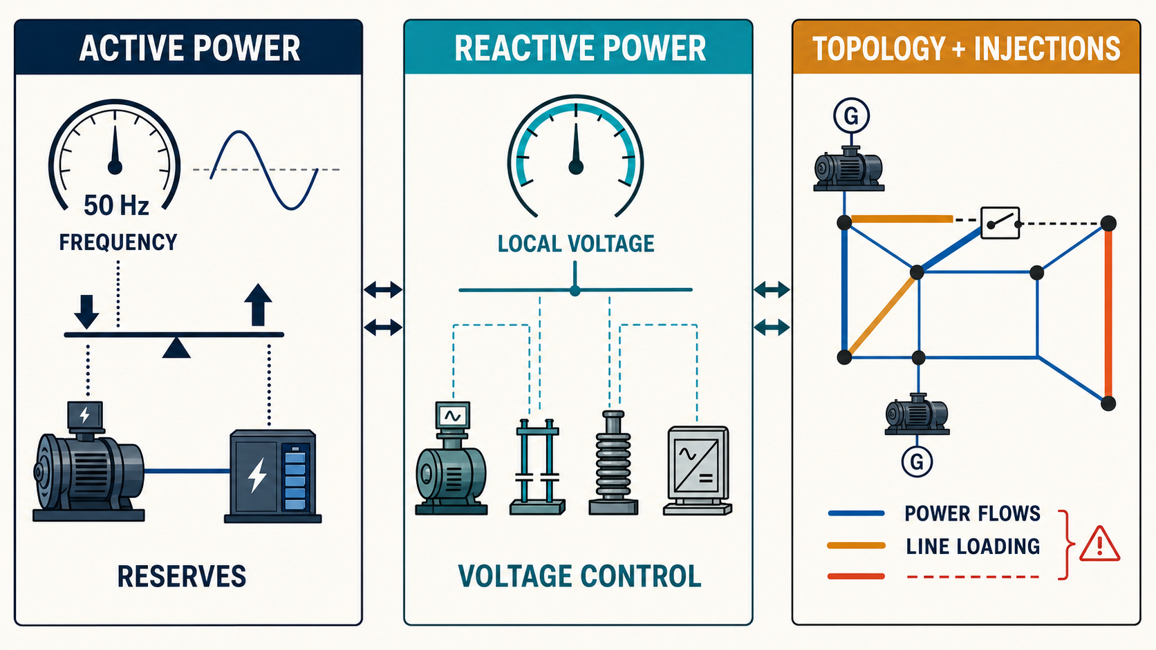
Figure 3: Operators manage several coupled problems at once. Active power strongly affects frequency, reactive power strongly affects voltage, and topology determines how both move through the network.
Power-flow control and redispatch
Operators cannot assign a route to each unit of power, but they can change the conditions that determine the flows.
Opening or closing selected breakers changes the topology. Transformer taps and phase-shifting transformers influence voltage and the distribution of active power. HVDC links can use controlled setpoints. Generation and consumption can be changed at specific locations.
One of the main tools is redispatch. A generator in one location increases output while another decreases output, keeping the total generation approximately balanced but changing where power enters the network.
Suppose a northern generator is increasing the loading of a constrained north-to-south corridor, while another plant closer to the southern load has spare capacity. Reducing the northern plant and increasing the southern plant can relieve the corridor without changing the total amount of generation.
Redispatch shows why a megawatt is not operationally identical in every location. The energy amount may be the same, but the effect on line loading, losses, voltage and contingency margins depends on where it is injected.
Normal Operation Is Already Active Work
A control room is not a fire brigade waiting for the next alarm. Normal operation requires continuous preparation because the safe state for the next hour may differ from the safe state now.
Demand follows daily and seasonal patterns but never matches a forecast exactly. Wind and solar output change with the weather. Generators start, stop and change output. International exchanges follow schedules while actual physical flows respond to the complete interconnected network. Equipment enters and leaves service for inspection, repair and construction.
Operators prepare switching programs before planned work. They confirm which breakers and disconnectors must change position, how the equipment will be isolated, what interlocks and safety procedures apply, and what the resulting topology means for the rest of the network.
An outage that is harmless during low demand may be unacceptable during a winter evening. Two individually reasonable maintenance plans may conflict because taking both assets out at once would remove the system’s ability to survive a further failure. This is why outage coordination extends across substations, companies and national borders.
The operator also watches operational limits. These include line and transformer loading, bus voltages, generator active and reactive capability, reserve availability, short-circuit levels and stability constraints. Some limits are immediate. Others permit a short overload while corrective action is prepared.
When analysis shows that one additional failure would violate a limit, the grid may enter an alert state even though all customers are still supplied and frequency is close to 50 Hz. The system is operating, but the safety margin has become too small.
The response might be preventive redispatch, returning an out-of-service line, changing topology, adjusting reactive-power resources, restricting a planned transfer or postponing maintenance. Good operation often looks uneventful because the risky state was corrected before a second event exposed it.
Coordination matters because the electrical system ignores organisational borders. A remedial action in one country can change flows in another. A distribution operator may control generators and reactive-power resources that affect the transmission grid. A power plant may own the machine, while the transmission operator is responsible for the wider system state. The EU System Operation Guideline formalises much of this data exchange and operational coordination between TSOs, DSOs and significant grid users.
A Large Generator Disconnects
We now have enough vocabulary to follow the failure from the opening example.
Assume a large synchronous generator is supplying 1,000 MW of active power and a meaningful amount of reactive power. A problem inside the plant causes its protection system to trip the unit and open the generator circuit breaker.
The exact numbers in the following sequence depend on the system state, but the order of responsibilities is stable.
The protection system disconnects the generator
The first action belongs to plant or generator protection. A relay detects a condition that makes continued connection unsafe, then commands the relevant circuit breaker to open.
This action protects the generator and the nearby electrical system. It may happen before the transmission control room knows that anything is wrong.
The breaker changes the topology. Active-power injection falls by 1,000 MW. The generator’s reactive-power contribution disappears as well. From that instant, the network has a new physical state.
Generation becomes lower than demand
Consumers have not coordinated with the failed plant. Their motors, heaters, trains and computers continue drawing power.
Total active-power generation is now lower than total active-power demand. The missing 1,000 MW is not supplied by one designated replacement generator during the first instant. The difference is initially supplied mainly by kinetic energy stored in the rotating masses of connected machines, while fast converter-based resources may also begin responding.
The electrical torque on the remaining synchronous generators becomes slightly greater than the mechanical torque supplied by their turbines. Their rotors slow down together, and the system frequency begins to fall.
This response is physical. No operator has selected it, and no SCADA command has caused it.
Local controls and FCR respond
Generator governors and other frequency-sensitive controllers detect the frequency change locally. Resources providing FCR begin increasing active-power injection or reducing consumption.
A hydro unit may open its guide vanes. A thermal unit may increase turbine input within its available headroom. A battery may inject power quickly. A pumped-storage plant may reduce pumping load. A flexible industrial consumer may lower demand.
These resources are distributed across the synchronous area. They do not need to know which generator failed. Frequency provides the common signal.
The reserve response grows while frequency is still falling. Eventually the additional power matches the deficit closely enough to stop the decline. The lowest point reached is called the frequency nadir.
If the response is sufficient, frequency stabilises. It may remain below 50 Hz because containment has stopped the movement without yet restoring the original balance.
Voltage and power flows change at the same time
The failed generator may have supported the voltage near its connection point. Losing its reactive-power capability can cause local voltage to fall, even while the frequency event is visible across the whole synchronous area.
Nearby automatic voltage regulators respond within their limits. Capacitors, reactors, converter controls or transformer taps may also act, depending on the network and configured control modes.
At the same time, active power begins entering the affected region from other generators through the transmission network. Flows redistribute across many lines. A corridor that previously carried moderate power may become heavily loaded because the local generator is no longer serving nearby demand.
This is where the graph from Part 2 becomes operational. The missing injection changes conditions across the network, and the most stressed line may be far from the failed plant.
Measurements and alarms reach the control centre
The generator breaker status changes. Active and reactive output measurements drop. Frequency values move. Nearby line flows and bus voltages change. Plant systems and substations create time-stamped events and alarms.
IEDs and RTUs forward this information through the operational communication network. SCADA updates the one-line diagram and alarm list. The operator may see a generator trip alarm, changed line colours, a frequency deviation and several secondary alarms caused by the same event.
These messages arrive after the physical system has already responded. They are evidence of the new state, not the trigger for the initial system-wide reaction.
Alarm handling is also harder than reading one clear error message. One event can produce hundreds of signals, some arriving out of order because different devices and communication paths have different delays. Operators and software need to distinguish the initiating event from its consequences.
State estimation and security analysis assess the new grid
The control centre now needs to answer several questions:
Was the generator the only element lost?
Are the received breaker states and measurements consistent?
Which lines and transformers are now more heavily loaded?
Has local voltage remained within its limits?
How much FCR and reactive-power capability is still available?
Can the grid survive the loss of another important component?
State estimation combines the new telemetry and topology with the network model. Power-flow and contingency-analysis applications calculate the current loading and simulate further outages.
The result may show that the frequency event is contained while the network is still unsafe. Perhaps one transmission corridor is close to its thermal limit. Perhaps local voltage is low. Perhaps the largest remaining generator has become the next critical contingency.
This is why returning frequency toward 50 Hz is necessary but insufficient. The full operating state must be secure.
aFRR and automatic generation control restore the area
FCR support came from across the synchronous area. The control area where the imbalance occurred must now restore its own balance and release that shared support.
The load-frequency controller calculates the control error from frequency and scheduled interchange. Through automatic generation control, it sends changing setpoints to resources providing aFRR.
These resources gradually add active power until the control-area imbalance is corrected. As aFRR takes over, FCR returns toward its neutral position and becomes available for the next disturbance.
If the outage lasts or the required correction is too large, mFRR and other slower actions replace part of the automatic response.
Operators create a new secure state
The failed generator may remain unavailable for hours. Operators cannot treat the restored frequency as the end of the incident.
They may redispatch generation so replacement power comes from locations that do not overload the network. They may start another plant, change pumped-storage operation, adjust cross-border schedules, switch reactive-power equipment, request new voltage setpoints or change the network topology.
They also need to restore reserve margins. A battery that delivered immediate power may need to recharge. Hydro and thermal units providing aFRR need room to respond in both directions again. The system should be able to survive another credible failure rather than remain balanced only while nothing else goes wrong.
The final state may look different from the state before the trip. A different set of generators is running, power flows use different corridors, reserve allocations have changed and some equipment may remain disconnected.
Recovery therefore means reaching a secure operating state, not recreating the exact previous state.
The same event on one timeline
Milliseconds: Protection detects the plant condition and trips the breaker. Local and automatic protection.
First electrical instant: Power flows change and rotating machines release stored energy. Physical response.
First seconds: Frequency-sensitive controls and FCR increase power or reduce load. Distributed automatic control.
Seconds to minutes: Telemetry, events and alarms reach SCADA; state estimation reconstructs the network. Monitoring and operational software.
Minutes: aFRR and automatic generation control restore the control area. Central automatic control.
Minutes to tens of minutes: mFRR, redispatch, voltage actions and topology changes establish a secure state. Automatic and operator-initiated control.
Hours and beyond: Rescheduling, reserve replenishment, investigation and repair continue. Operation and asset management.
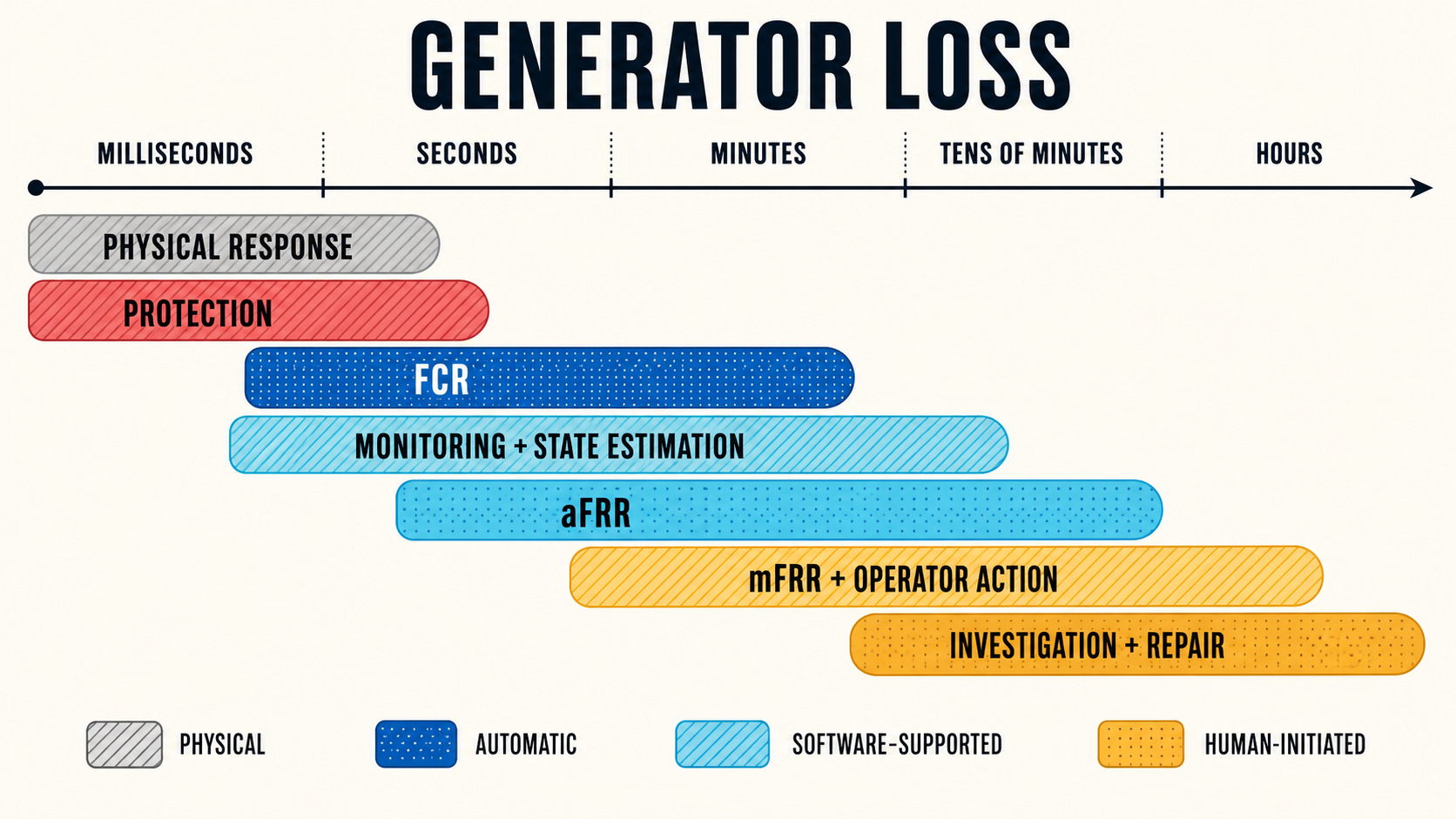
Figure 4: A generator loss is handled by several overlapping layers. Physics and local automation contain the first moments, while central controls and operators rebuild a secure system.
If the Normal Response Is Not Enough
The scenario above ends well because the protection system isolates the plant cleanly, reserves are sufficient and the network has enough remaining capacity.
A larger event, several simultaneous outages or a weak initial state can exhaust those layers.
If frequency continues falling, automatic under-frequency schemes can disconnect blocks of load. Removing consumers is damaging, but it can rebalance an island or synchronous area before generators also disconnect and the entire system collapses.
If voltage keeps falling, operators and automatic schemes may use all available reactive-power support, block transformer tap changers, reduce voltage targets or disconnect demand. If power flows remain outside safe limits, equipment may be switched, generation may be redispatched, transfers may be reduced and, in an emergency, selected loads may be disconnected.
These measures are defined in system defence plans. The European framework for emergency and restoration operation is set out in Regulation (EU) 2017/2196.
Protection still has a difficult role. If an overloaded line trips, its flow redistributes over the remaining network. Another line may then exceed its limit and trip as well. Each relay may be correctly protecting its own asset while the sequence weakens the wider system.
This is the basic mechanism behind a cascading outage:
One element disconnects.
Flows and voltages redistribute.
Another element exceeds its limits.
Protection disconnects it.
The remaining network receives even more stress.
The grid may eventually split into electrical islands. Each island must immediately balance its own generation and load. An island with too little generation experiences falling frequency, while an island with too much generation experiences rising frequency.
Emergency controls attempt to stop the cascade, preserve stable islands and keep as much of the system supplied as possible.
Different Disturbances Stress Different Layers
The generator loss gives us a useful complete story, but it should not become a template for every event.
A transmission line fault begins with a short circuit or another abnormal electrical condition. Line protection detects the fault and opens breakers at one or both ends, often within a fraction of a second. Generation and demand may remain nearly balanced, so the initial frequency change can be small, while the main operational problem is redistributed power flow and reduced transmission margin.
A transformer outage can remove the connection between voltage levels or parts of a substation. The result may be a local supply problem, overloaded parallel transformers, changed short-circuit levels or a voltage issue rather than a large system-wide frequency event.
A sudden rise in reactive-power demand, perhaps from large motors or a heavily loaded region, can depress local voltage while total active-power generation still matches consumption. Frequency can remain close to 50 Hz while part of the network approaches voltage instability.
A regional separation creates the clearest example of the system’s coupled nature. Once tie lines open, the two sides no longer share one active-power balance. Each island follows its own imbalance and frequency trajectory.
Protection, monitoring, operation and control appear in every case, but their order and relative importance change with the physical disturbance.
Where the Distributed-Systems Analogy Helps
We can now return to the failed data centre.
Both systems need observability. Operators need trustworthy measurements, event histories, health information and models that explain what is connected and available.
Both need spare capacity. A service without compute headroom cannot absorb traffic from a failed region. A grid without active-power reserves, reactive capability or transmission margin cannot absorb an electrical outage safely.
Both use layered response. Local components handle some failures automatically, central systems coordinate wider recovery, and human operators intervene when the event crosses the assumptions built into automation.
Both can operate in a degraded state. A service may remain available with higher latency and reduced redundancy. A grid may restore frequency while running with tighter transmission margins and less reserve.
Both need to prepare for the next failure. Recovering the current workload is not enough if the platform has lost all remaining redundancy. Restoring generation-load balance is not enough if the grid can no longer survive another contingency.
These similarities make distributed systems a useful starting point for developers entering the energy industry.
Where the Analogy Stops
The limitations matter just as much.
Software work can often be queued. Electrical load continues interacting with the network at every instant.
Software traffic can be assigned to a region or route. AC power divides across the connected network according to impedance, voltage and phase angle.
Many software failures remain local until another component calls the failed service. An electrical disconnection changes the physical state of the wider network immediately.
A monitoring system in software may detect a problem before users notice it. In the grid, frequency, voltage and current may already be moving before the control centre receives the first event.
Software replicas can disagree temporarily while eventual consistency resolves the difference. The synchronous grid has shared physical variables that must remain inside narrow limits continuously.
Finally, grid control actions feed back into the same physical system being measured. Opening a breaker to remove an overload changes flows elsewhere. Raising a downstream voltage can increase demand on an upstream network. Increasing one generator can relieve frequency while worsening congestion.
This is why grid software cannot be designed only as ordinary enterprise software with stricter availability requirements. It participates in a control loop around a large physical machine.
The Mental Model to Keep
A developer does not need to become a protection engineer or a control-room dispatcher to understand where grid software fits. The following model is enough to organise the vocabulary:
Physics moves first. Changes in generation, load or topology immediately affect frequency, voltage, current and power flow.
Protection removes immediate danger. Relays and circuit breakers isolate faults locally and quickly.
Monitoring constructs visibility. Field measurements, substation devices, communications, SCADA and state estimation create an operational picture.
Control changes the system. Governors, voltage regulators, reserves, automatic generation control, tap changers, reactive-power devices, redispatch and switching move the grid toward acceptable conditions.
Operation chooses and coordinates the secure state. Dispatchers assess limits, contingencies, outages and available actions across organisational and national boundaries.
None of these layers works alone. Protection can clear a fault but cannot replace lost generation. SCADA can show an overload but cannot decide which market and operational constraints matter. Reserves can restore active-power balance but cannot help if the replacement power has no safe transmission path. Operators cannot act effectively when measurements or models are wrong.
The European grid stays stable because these layers overlap across different timescales. Local physics and automation handle the first instant. Wide-area controls restore balance. Software helps operators understand the changing state. Human decisions rebuild enough margin for the next event.
In Part 1, we assembled the electromagnetic machine. In Part 2, we assembled the graph. Here, the graph became operational.
It is always changing, always measured and always being corrected. Stability is the result of that continuous work.
Next part:

All parts of the series:
